This is an analysis of the Britich Family Incomes (from a survey of ~7000 families in 1975), using histograms.  It illustrates some of the potential pitfalls of histograms for visualizing data.
 

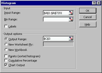
First the data were entered into an Excel Spreadsheet.  Use   Tools   --->    Data Analysis    --->    Histogram, to pull up the Histogram menu.

The fields have been filled out so that:

    -  The range of the input data is in the "Input Range" box (see Class Example 1 for details of ways to do this).

    -  Leaving the "Bin Range" box blank, instructs Excel to choose its own bin range.  To choose your own bins, first create a column of bin boundaries, and then put that range into this box.

    -  The "Output Range" box is filled out with a blank cell, where Excel will write the bin boundaries, and the bin frequencies.

    -  The "Chart Output" box is checked, so that Excel will make a picture of the resulting histogram (versus just computing the frequencies).

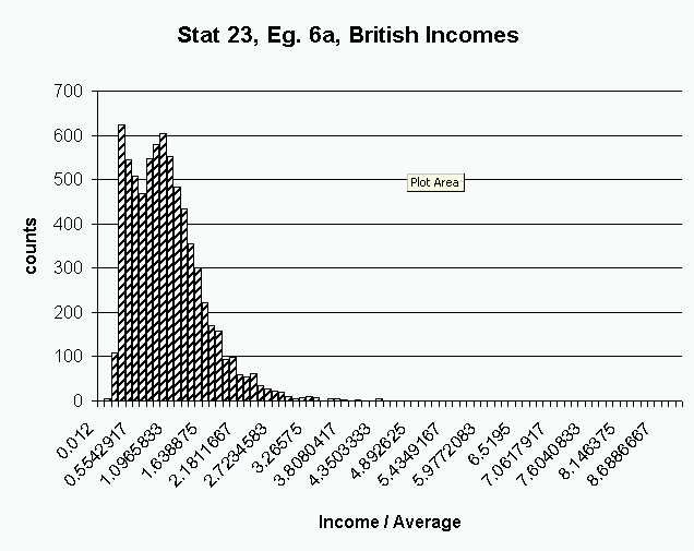
Here is resulting histogram.  The bins were chosen by Excel.  Some of the graphics have been improved for this type of display, e.g. the bars have been made full width)
:
The shape of the distribution is what one would expect from income.  Most of the population has fairly low to moderate income.  A few people earn much more than the rest of the population.  Such a distribution is called "heavy tailed" and "skewed to the right".
 

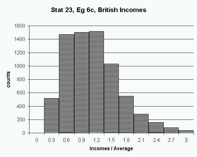
    Since almost all of the data is between 0 and 3, this view is wasteful in the sense of not making good use of the graphics space available.  To better use the available space, only the data points less than 3 are put into the Histogram tool:

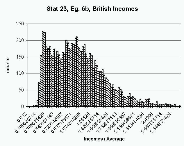
This histogram looks "rough", because the binwidth is too small (good default choices are not easy to find, and there is not a consensus about what is the "right" way to do this).  A perhaps too large amount of "sampling variability" appears in this histogram.
 

To choose your own (thus different from that chosen by Excel) binwidth, create a vector of bin boundaries (recall, create the first two, highlight them together, and drag downwards on the litle black box in the corner), and insert its range (see Class Example 1 for details about this)  in the "Bin Range" box of the Excel Histogram menu.

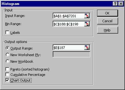
Here is the resulting Histogram, using a much bigger binwidth.  First, the bin boundaries are created in Excel, then put into the Histogram menu:

Here that binwidth is so large that it obscures the "two bumps" that were visible above.  An interesting question is whether or the two bumps represent important underlying structure, or are just noise artifacts.  This question is answered (they really are there) for example in the paper:

Schmitz, H. P. and Marron, J. S. (1992) “Simultaneous estimation of several size distributions of  income”,  Econometric Theory, 8, 476-488.
 

Here is a perhaps better binwidth, which represents a trade off between getting the important structure, without too much sampling noise appearing:

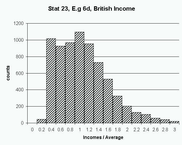
Note that the two bumps are both visible, and the shape is quite smooth elsewhere.
 

The width of the bins affects has a strong effect on what is seen in a histogram.  Perhaps more surprising is the bin location can also have quite an important effect.  To see this, consider the following histogram which uses the same binwidth as the example just above:

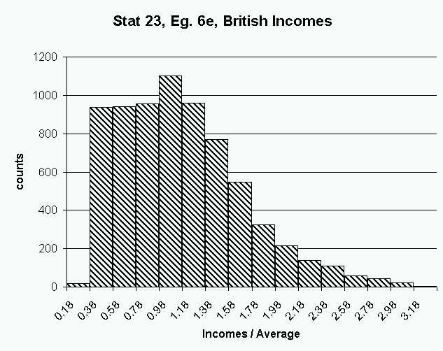
Note that the important "two bump" sturcture has disappeared!  It happened by just "sliding the histogram grid" over just a little bit to the left.  For this reason, care needs to be taken in the use of histograms.  In particular, several binning grids should be considered.
 
 

The final result of all the work done here is available on the spread sheet version of this example.
 
 

Back to Stat 23 Home Page
 

Back to Marron's Home Page