This is a step by step solution Homework Problem 3.11 from the textbook, using Excel.
 

Answer to Part a of Exercise 3.11:

Each of the companies listed in the table is one sample point.
 
 

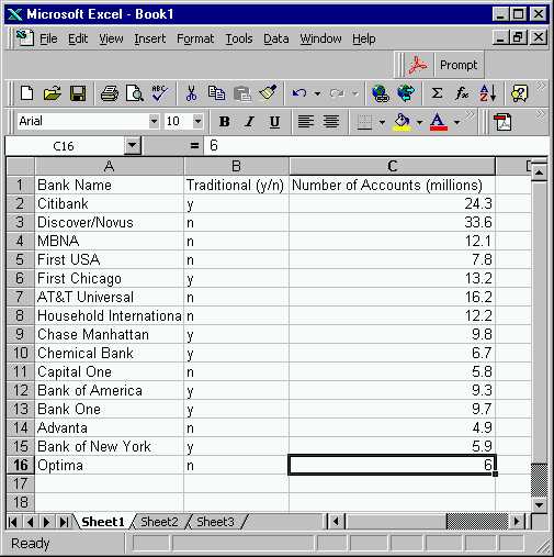
Step 1:  Type the data into an Excel spreadsheet.  Here is the result:

Note that the top row are "headers" that help remember (if you go back to look at this later) what is in each column.  Also note that the columns have been widened, for easier viewing.  This can be done by putting the mouse cursor right between two columns, holding down the left mouse button, and moving the column boundary.
 

Step 2:  Put the total for column C at its base.  For this first highlight the empty box just below that shown above.  Then use menus  "Insert"    "Function..."  which pulls up the "Paste Function" menu:.

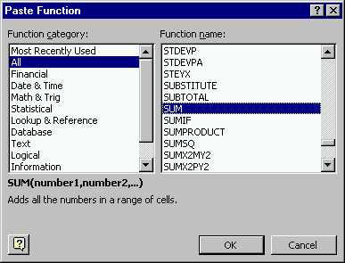
Next, highlight choices as shown above (moving sliders on the right edges as needed), and choose OK.  This pulls up the menu:

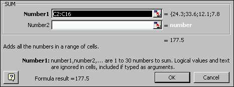
Note that Excel automatically chose the range of cells above (it made a good guess about we wanted to sum, based on what was highlighted).  Here are some ways to get the right range in boxes like this (e.g. when Excel doesn't make a good guess):

    i.     Sometimes (but far from always) you can highlight the range you want before you pull up the menu, and that becomes Excel's guess.

    ii.    Just type the indices of the desired range into the box.  You should be very comfortable with this approach, as it will be tested on exams.

    iii.   Click the little blue, red and white square just at the right edge of the box.  This pulls up a very thin menu, which will show the range for the area that you highlight with the mouse.  Go to the spreadsheet and highlight the range that you want (Note instead of the usual thick black boundary for the highlight, you now get a moving striped boundary).  If part of range that you want isn't visible, use the controls bars at the side and bottom to move the sheet around. When you get the range you want, click the little colored square at the right edge of the thin menu

More than one box is allowed in case you want to sum over other types of range.

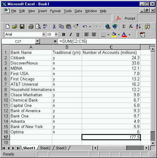
Next Choose OK, and note that the total appears at the foot of Column C:

Step 3:  Add a new column D, where the entries in Column C are divided by the total for Column C.  Do this by highlighting the box D2, and typing in the formula "=C2/$C$17"  (do this EXACTLY, e.g. if you forget the "=", Excel thinks you are giving it a string of characters).  The "$C$17", gives an "absolute reference, which is needed as discussed below).  When you hit "Enter", it looks like this:

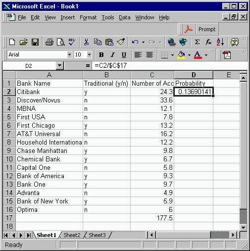
Note the entered formula appears near the top (you can change this at any time if you like), and the number is the result of dividing the C2 entry by the C17 entry.  Now extend the formula to the whole D column, but dragging the tiny square in the lower right corner of the highlighted box downwards, to get:

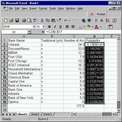
These numbers sum to 1 (try this using the above steps), and thus can be viewed as probabilities (hence the choice of column header).  These are the probabilities of each company being chosen, when a random account is chosen.
 
 

Answer to Part b of Exercise 3.11:

The probabilities for each sample point, i.e. each company, are given in column D.
 
 

Step 4:  Find the probability of a randomly chosen account coming from a nontraditional bank, by summing the probabilities over the nontraditional banks.  A convenient way of doing this is with the command "sumif".  This can either come from the "Insert,    Function..." menus as above, or can be just typed in.  In either case, you end up with:

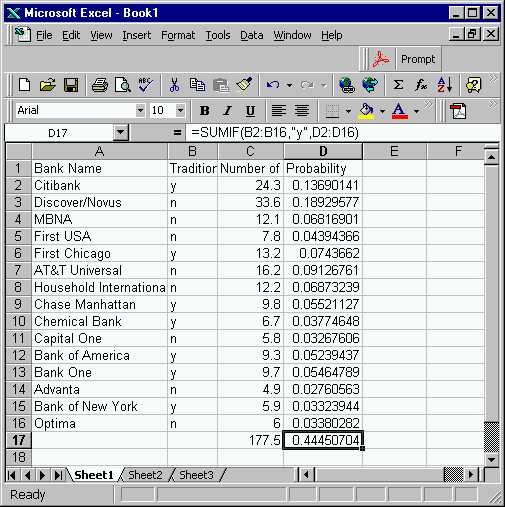
Answer to Part c of Exercise 3.11:

The probability that a randomly chosen account is from a traditional bank is 44.5%
 
 

Back to Stat 23 Home Page
 

Back to Marron's Home Page