a. Assuming "New heavy tail duration", Version 1: For some
from Cornell Course OR778,
Fall semester, 2001
1. (from Lecture9-3-01) For Q-Q plots, turn visual tool of "simulated envelope to assess variability" from:
For example, how can one use this to define a p-value?
Challenges:
-
correct handling of simultaneous inference
-
incorporating variability of parameter estimation
2. (from Lecture9-5-01) Is "non-stationarity" observed in moving window (of 50,000) Q-Q analysis of Response Size data:
A related question:
3. (from Lecture9-5-01)
How does Q-Q analysis change, if replaced by:
-
Hill (maximum likelihood) estimation (suitably truncated)?
-
least squares fit of line to suitable range of quantiles?
4. (from Lecture9-5-01)
Find a "good", precise mathematical definition of:
"heavy tailed" distributions
Some ideas:
-
not moment based
-
should depend on "range of interest"
-
empirical version depends on sample size
-
not a number, but a "curve"?
-
what will it be used for??
5. (from Lecture9-10-01)
How can "Long Range Dependence" be measured for heavy tailed distributions?
6. (from Lecture9-10-01)
Show that the Pareto distribution is visually more variable for heavier
tails (i.e. the envelope shown in the Pareto
Q-Q plots expands for heavier tails)
7. (from Lecture9-10-01)
Do a formal hypothesis test of "heavy tails" (i.e. shape parameter <
2, over a wide range of quantiles) for the Response Size data.
8. (from Lecture9-10-01)
How can variability be assessed (even visually) in a CDF plot?
9. (from Lecture9-26-01)
for mice and
elephant
plots, use "length biased" sampling and "truncated
data" ideas:
- to explore correctness of 80% window view
- to correctly modify smaller window views
- to find "best view"
10.
(from Lecture10-03-01)
which of the following can explain the strong mean changes observed in
the start time SiZer
analysis?
a. Independent
Weibull(0.9) interarrivals?
b. Poisson
cluster process?
11.
(from Lecture10-17-01)
a. What
is the Residual Life Distribution for the log normal?
b. Again
log normal, or different shape?
c. Can
this give new insights regarding the controversy (of Pareto vs. logNormal
distributions)?
d. If
data are log normal, and a Pareto is fit to two quantiles,
will the residual life time distribution still have the correspondingly
adjusted Pareto fit?
12.
(from Lecture10-17-01
and Lecture 11-26-01)
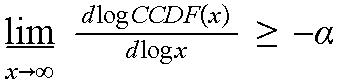
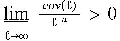
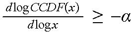
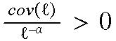
a. Assuming
"New heavy tail duration", Version 1: For some ![]() ,
,
 ?
? "most of the time" (in some sense)? Also assuming
the simple model,
"most of the time" (in some sense)? Also assuming
the simple model,
 (in a suitable sense)?