The t-distribution, and using Excel to calculate t probabilities.
 

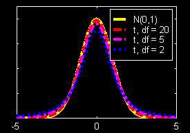
First look at how the t distribution compares to the Standard Normal distribution:

These are probability density curves. Remarks:
  -  The t densities also have a mound shape, fairly similar to the normal.
  -  They are all "more spread", and the spreading is more
                        for larger degrees of freedom.
  -  The "small probability cutoffs" will be much farther out
                        for smaller degrees of freedom.
  -  The t curves converge to the Normal curve as the
                        degrees of freedom goes to infinity.
 

The main idea is to use     Insert    --->    Function     --->    TDIST

(e.g. in the "Statistical" section of the "Paste Function" menu, or alternatively get to here using the "f sub x" button) as a replacement for NORMDIST;.

Similarly use TINV in place of NORMINV.
 

The big picture organization of these is:

These functions allow conversion between cutoff and Area as:

1.  To get Area, from a given cutoff, use:
             Area = NORMDIST(cutoff, [& other params])
             Area = TDIST(cutoff, [& other params])

2.  To get cutoff from a given "Area", use:
            cutoff  = NORMINV(Area, [& other params])
            cutoff  = TINV(Area, [& other params])
 

Eg 14.1:     For  T ~ t(15), i.e, "T has a Student's t distribution, with n degrees of freedom",  find  P{T < 1.41}.

This problem is of the type 1 above.

Use the above steps to arrive at the TDIST menu.  Fill out the menu as usual, using either typed in numbers, or references to cells, to get:

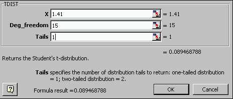
Notes:
  -  the cutoff here is "x", set to 1.41.
  -  the degrees of freedom (reflecting variability in s) is set to 15.
  -  the "tails" parameter is new.  Set this to one, since we don't want both tails here.
  -  the final probability is 0.0895.

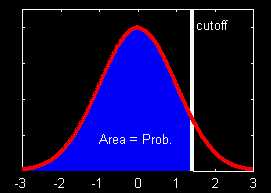
CAREFUL:  that final probability is way off.  Here is the picture of what we are after:

This probability is clearly much bigger than 0.5 (in contrast to the above answer of ~0.09).

The lesson is that TDIST works in a different way from NORMDIST.  In particular, it works with tails of the distribution.  So to calculate this probability, the "1 -" approach needs to be used. Here is the resulting spreadsheet with the correct answer:

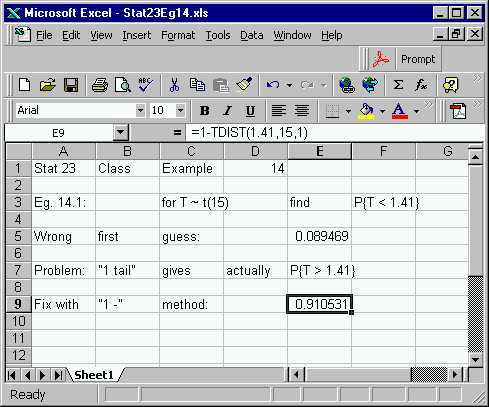
Notes:
  -  this answer is much more sensible
  -  the formula bar shows how to work with this by just typing in a formula
                                  (this skill will be needed for the midterm).
  -  the corresponding Standard Normal probability, P{Z < 1.41} = 0.921
                                  is rather close, and larger (as expected from above pic)
 

Eg 14.2:     For  T ~ t(5),  find  P{0.02 < T < 1.41}.

This is done using the same idea as for Normals:
P{0.02 < T < 1.41}  =  P{0.02 < T}  -  P{1.41 < T}  =
                                 =  "=TDIST(0.02,5,1) - TDIST(1.41,5,1)"
                                 =  0.384

Notes:
  -  the probabilities "go the other way", because of the "tail" aspect of TDIST.
  -  Once again this is close to the corresponding N(0,1) version:
                                    P{0.02 < Z < 1.41}  =  0.413
             but the gap is bigger this time, since the degrees of freedom is smaller
                                                        (thus farther from the Standard Normal)
 

Eg 14.3:     For  T ~ t(60),  find  P{|T| < 1.96}.

Recall that this can also be written as:
          P{|T| < 1.96}  =  P{-1.96 < T < 1.96}

The picture for this one is:

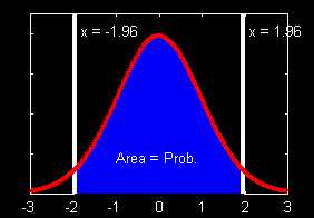
Here is where the "2-tail" option of TDIST is really useful.  Instead of the serious fiddling with areas that is needed for NORMDIST, this is now much easier.

But recall that "tails" means "the outside part", so use the "1 -" trick:
          P{|T| < 1.96}  =  1 - P{|T| > 1.96}
                                  =  1 - TDIST(1.96,60,2)
                                  =  0.945

Again it is interesting to compare to the Normal.  For this large degrees of freedom, expect close answers, and indeed get:
          P{|Z| < 1.96}=  0.950
 

Eg 14.4:     For  T ~ t(13),  find  c  so that  P{|T| > c}  =  0.10.

Note that this is now a problem of the type 2, in the general setup above, so use TINV.

The TINV menu, appropriately filled out is:

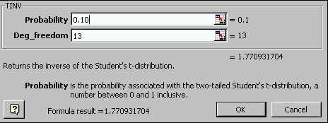
Notes:
  -  Here one must use the 2-tailed version, (there is no one tailed option).
  -  The answer is once again close to (and as expected slightly larger than)
                                             the Standard Normal answer:  1.64
 

Eg 14.5:     For  T ~ t(7),  find  c  so that  P{T > c}  =  0.10.

This one is harder than the above, since TINV works only in two tailed terms.  The trick is to rewrite the problem in terms of a 2 tailed probability:
   P{|T| > c}  =  P{T < -c   or   c < T}  =
                     =  P{T < -c}  +  P{c < T}  =                  (since events are disjoint)
                     =  P{T > c}  +  P{T > c}  =                   (using symmetry of the t dist.)
                     =  2 * P{T > c}

Thus want to find  c  so that:
   P{|T| > c}  =  0.20

Get this by:   TINV(0.2,7)  =  1.41
 

The final result of all the work done here is available on the spread sheet version of this example.
 
 

Back to Stat 23 Home Page
 

Back to Marron's Home Page