Using Excel to calculate Normal (Gaussian) probabilities.
 

The main idea is to use     Insert    --->    Function     --->    NORMDIST     (e.g. in the "Statistical" section of the "Paste Function" menu).

Recall that you often use a shortcut of pushing the "f sub x" button on a bar near the top.
 

Eg 11.1:     For  Z ~ N(0,1),  find  P{Z < 1.41}.

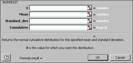
Use the above steps to arrive at the NORMDIST menu:

 

Fill these out using either typed in numbers, or references to cells, to get:

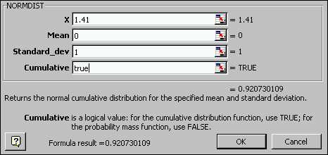
Note:  the "cumulative" works in a fashion similar to the Binomial, except that we will basically always use "true".  The only time we will use "false" is if we need to produce a plot of the Normal density (called "mass") function (i. e. the underlying "mound shaped curve").
 

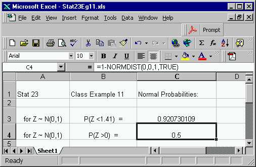
Click "OK" to get the answer:

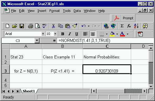
As with other Excel functions, you can either use the menu to get this probability, or else you can just type the formula "=NORMDIST(1.41,0,1,TRUE)" into the formula bar.  Also any of the arguments can be modified, to include ranges (absolute or relative).
 

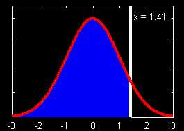
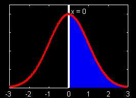
For the coming harder problems, it is often useful to think of such probabilities in terms of a plot of the corresponding areas.  Here is the area plot for this simplest problem:

 
 
 

Eg 11.2:     For  Z ~ N(0,1),  find  P{Z >0}.

Similar to what happened for the Binomial, Excel does not give probabilities of this form (it works in terms of  Z <,  not Z >,  as needed here).  The solution is the same:  use rules of probability to put the answer into the needed form:

P{Z>0} = 1 - P{Z < 0}      (recall don't need to worry about Z = 0 for continuous random variables)

The just put that directly into Excel (you can use the menu as above, or you copy what is in box C3, and modify it on the formula bar):

Note the answer of 0.5 can also be derived by using the symmetry of the distribution, as seen in the area plot:

 
 

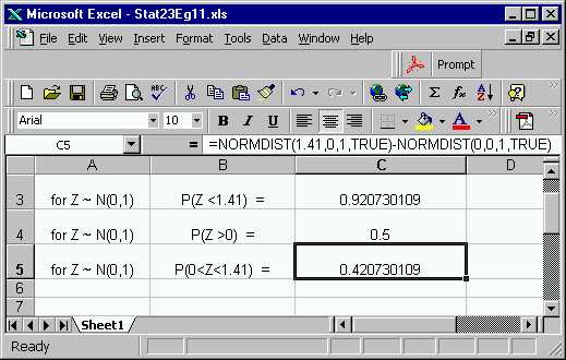
Eg 11.3:     For  Z ~ N(0,1),  find  P{0 < Z < 1.41}.

The key idea here is again the same as what we did with the Binomial, i.e. do some manipulation, to put probabilities into a form that can be handled by Excel:

P{0 < Z < 1.41} = P{Z < 1.41} - P{0 < Z}

So the answer is just the difference of the two probabilities calculated above:

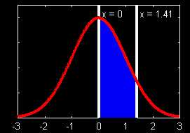
Many people obtain insight from thinking of this operation in a graphical way:

  -   = 
 
 
 

Often it will be useful to "solve equations involving probabilities":

Eg 11.4:   For  Z ~ N(0,1), find the number c, so that 0.68 = P{Z < c}.

One way to solve this would be by simple trial and error.  E.g. one could just try some c values in the Excel NORMDIST function, using successively larger values depending on the calculated probability, until a c value is found that gives the desired answer.  A slightly quicker, very similar, approach would be to just try a range of c values:

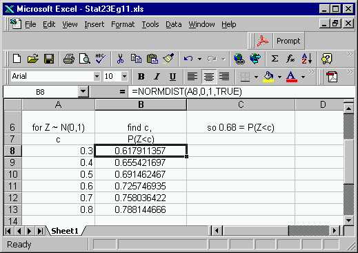
Note that this time the NORMDIST function was used with a cell reference, in the usual way.

The desired value of 0.68 is between the probs for  c = 0.4  and  c = 0.5.  More precision can be obtained by using a finer grid of  c  values.  However, this seems like the sort of thing that a computer should be able to do automatically, and indeed Excel has a function which does essentially this.  Such a function gives the mathematical "inverse" of NORMDIST, so it is called NORMINV.  Here is the NORMINV menu, which is filled out in the usual way:

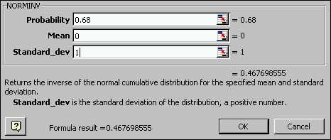
This gives the answer:

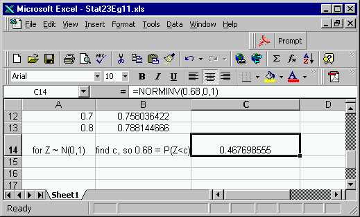
Note this answer seems sensible with respect to the table of c values given above (i.e. between 0.4 and 0.5).

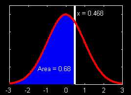
Basically the same graphic as above adds insight to this problem:

 
 
 

Summary:  NORMDIST and NORMINV give both sides of the relationship between "numbers on the axis", and "areas under the Normal curve".

Use NORMDIST     to go from    "numbers on axis"     to     "areas"

Use NORMINV     to go from    "areas"     to    "numbers on axis"
 

To work with an arbitrary (i.e. not necessarily "standard") Normal distribution, do the same type of thing, but use the given values of the mean and the standard deviation.

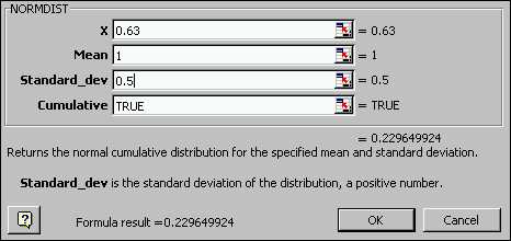
Eg 11.5:     For  X ~ N(1,0.5),  find  P{X < 0.63}.

Here is the NORMDIST menu:

 

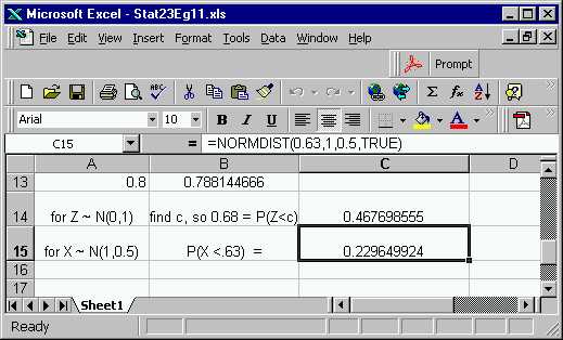
Which gives the result:

 

Again there is a corresponding graphic:

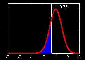
Note that this Normal(1,0.5) curve is moved to the right, and narrower, in comparison to the standard normal curves used above.
 

As for the Standard Normal examples above, there are parallel examples of other types for general mean and standard deviation versions.  They are worked out in the same way.
 
 

The final result of all the work done here is available on the spread sheet version of this example.
 
 

Back to Stat 23 Home Page
 

Back to Marron's Home Page